1. 基本xy平面绘图命令
MATLAB不但擅长於矩阵相关的数值运算,也适合用在各种科学目视表示(Scientific visualization)。
本节将介绍MATLAB基本xy平面及xyz空间的各项绘图命令,包含一维曲线及二维曲面的绘制、列印及存档。
plot是绘制一维曲线的基本函数,但在使用此函数之前,我们需先定义曲线上每一点的x 及y座标。
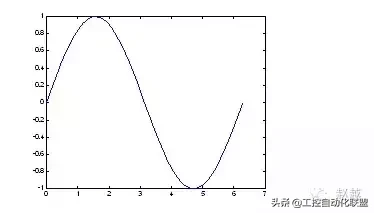
下例可画出一条正弦曲线:
close all;
x=linspace(0, 2*pi, 100); % 100个点的x座标
y=sin(x); % 对应的y座标
plot(x,y);
小整理:MATLAB基本绘图函数
plot: x轴和y轴均为线性刻度(Linear scale)
loglog: x轴和y轴均为对数刻度(Logarithmic scale)semilogx: x轴为对数刻度,y轴为线性刻度
semilogy: x轴为线性刻度,y轴为对数刻度
若要画出多条曲线,只需将座标对依次放入plot函数即可:
plot(x, sin(x), x, cos(x));
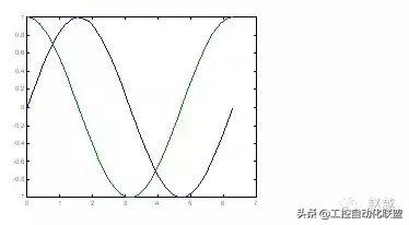
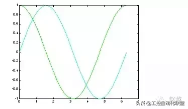
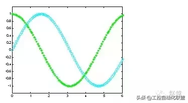
若要改变颜色,在座标对後面加上相关字串即可:
plot(x, sin(x), 'c', x, cos(x), 'g');
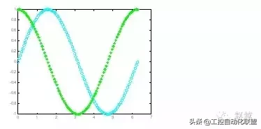
若要同时改变颜色及图线型态(Line style),也是在座标对後面加上相关字串即可:
plot(x, sin(x), 'co', x, cos(x), 'g*');
小整理:plot绘图函数的叁数字元颜色字元图线型态y 黄色。点k黑色o 圆w 白色x xb 蓝色+ +g 绿色* *r 红色- 实线c 亮青色: 点线m 锰紫色-. 点虚线-- 虚线图形完成後,我们可用axis([xmin,xmax,ymin,ymax])函数来调整图轴的范围:
axis([0, 6, -1.2, 1.2]);
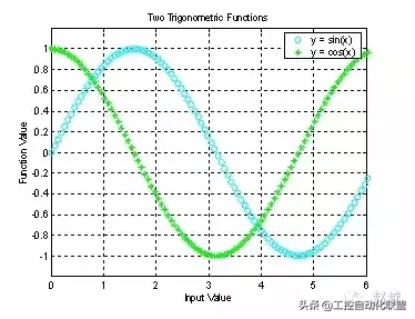
此外,MATLAB也可对图形加上各种注解与处理:
xlabel('Input Value'); % x轴注解
ylabel('Function Value'); % y轴注解
title('Two Trigonometric Functions'); % 图形标题
legend('y = sin(x)','y = cos(x)'); % 图形注解
grid on; % 显示格线
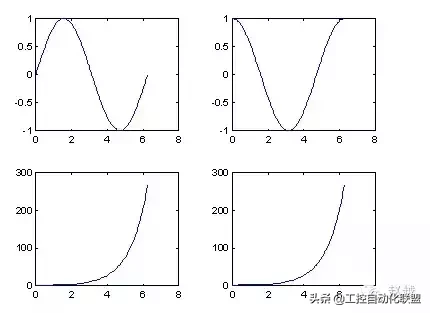
我们可用subplot来同时画出数个小图形於同一个视窗之中:
subplot(2,2,1); plot(x, sin(x));
subplot(2,2,2); plot(x, cos(x));
subplot(2,2,3); plot(x, sinh(x));
subplot(2,2,4); plot(x, cosh(x));
MATLAB还有其他各种二维绘图函数,以适合不同的应用,详见下表。
小整理:其他各种二维绘图函数
bar 长条图
errorbar 图形加上误差范围
fplot 较精确的函数图形
polar 极座标图
hist 累计图
rose 极座标累计图
stairs 阶梯图
stem 针状图
fill 实心图
feather 羽毛图
compass 罗盘图
quiver 向量场图
以下我们针对每个函数举例。
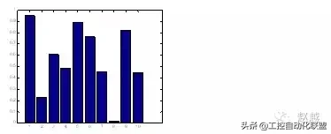
当资料点数量不多时,长条图是很适合的表示方式:
close all; % 关闭所有的图形视窗
x=1:10;
y=rand(size(x));
bar(x,y);
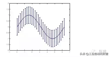
如果已知资料的误差量,就可用errorbar来表示。下例以单位标准差来做资的误差量:
x = linspace(0,2*pi,30);
y = sin(x);
e = std(y)*ones(size(x));
errorbar(x,y,e)
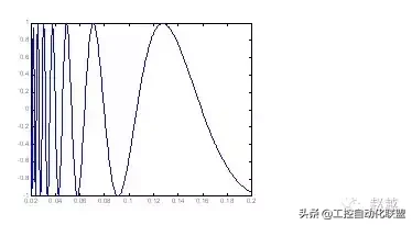
对於变化剧烈的函数,可用fplot来进行较精确的绘图,会对剧烈变化处进行较密集的取样,如下例:
fplot('sin(1/x)', [0.02 0.2]); % [0.02 0.2]是绘图范围
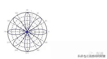
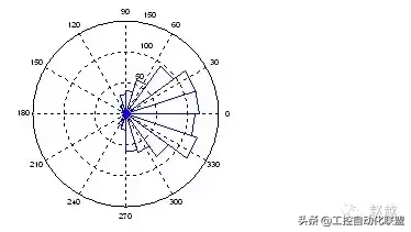
若要产生极座标图形,可用polar:
theta=linspace(0, 2*pi);
r=cos(4*theta);
polar(theta, r);
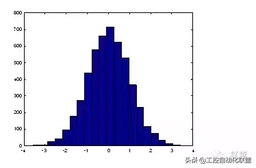
对於大量的资料,我们可用hist来显示资料的分 情况和统计特性。下面几个命令可用来验证randn产生的高斯乱数分 :
x=randn(5000, 1); % 产生5000个 m=0,s=1 的高斯乱数
hist(x,20); % 20代表长条的个数
rose和hist很接近,只不过是将资料大小视为角度,资料个数视为距离,并用极座标绘制表示:
x=randn(1000, 1);
rose(x);
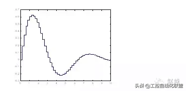
stairs可画出阶梯图:
x=linspace(0,10,50);
y=sin(x).*exp(-x/3);
stairs(x,y);
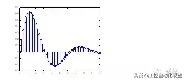
stems可产生针状图,常被用来绘制数位讯号:
x=linspace(0,10,50);
y=sin(x).*exp(-x/3);
stem(x,y);
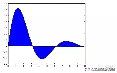
stairs将资料点视为多边行顶点,并将此多边行涂上颜色:
x=linspace(0,10,50);
y=sin(x).*exp(-x/3);
fill(x,y,'b'); % 'b'为蓝色
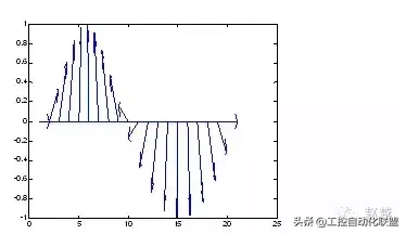
feather将每一个资料点视复数,并以箭号画出:
theta=linspace(0, 2*pi, 20);
z = cos(theta)+i*sin(theta);
feather(z);
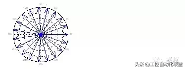
compass和feather很接近,只是每个箭号的起点都在圆点:
theta=linspace(0, 2*pi, 20);
z = cos(theta)+i*sin(theta);
compass(z);
2.基本XYZ立体绘图命令
在科学目视表示(Scientific visualization)中,三度空间的立体图是一个非常重要的技巧。本章将介绍MATLAB基本XYZ三度空间的各项绘图命令。
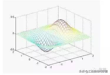
mesh和plot是三度空间立体绘图的基本命令,mesh可画出立体网状图,plot则可画出立体曲面图,两者产生的图形都会依高度而有不同颜色。
下列命令可画出由函数<图片>形成的立体网状图:
x=linspace(-2, 2, 25); % 在x轴上取25点
y=linspace(-2, 2, 25); % 在y轴上取25点
[xx,yy]=meshgrid(x, y); % xx和yy都是21x21的矩阵
zz=xx.*exp(-xx.^2-yy.^2); % 计算函数值,zz也是21x21的矩阵
mesh(xx, yy, zz); % 画出立体网状图
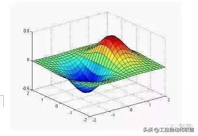
surf和mesh的用法类似:
x=linspace(-2, 2, 25); % 在x轴上取25点
y=linspace(-2, 2, 25); % 在y轴上取25点
[xx,yy]=meshgrid(x, y); % xx和yy都是21x21的矩阵
zz=xx.*exp(-xx.^2-yy.^2); % 计算函数值,zz也是21x21的矩阵
surf(xx, yy, zz); % 画出立体曲面图
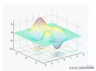
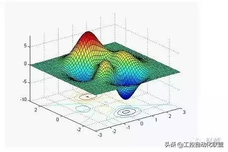
为了方便测试立体绘图,MATLAB提供了一个peaks函数,可产生一个凹凸有致的曲面,包含了三个局部极大点及三个局部极小点要画出此函数的最快方法即是直接键入peaks:
peaks
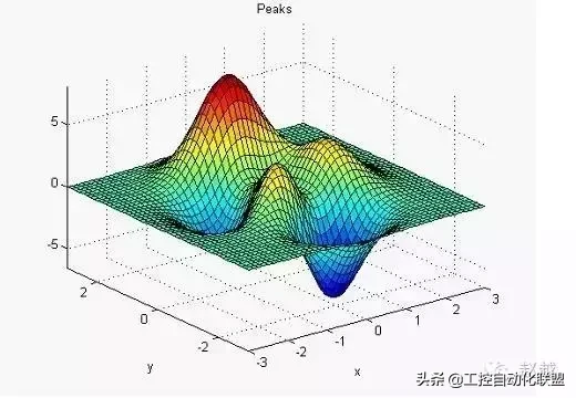
z = 3*(1-x).^2.*exp(-(x.^2) - (y+1).^2) ...
- 10*(x/5 - x.^3 - y.^5).*exp(-x.^2-y.^2) ...
- 1/3*exp(-(x+1).^2 - y.^2)
我们亦可对peaks函数取点,再以各种不同方法进行绘图。
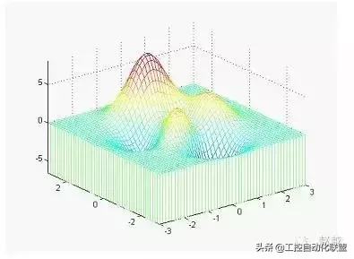
meshz可将曲面加上围裙:
[x,y,z]=peaks;
meshz(x,y,z);
axis([-inf inf -inf inf -inf inf]);
waterfall可在x方向或y方向产生水流效果:
[x,y,z]=peaks;
waterfall(x,y,z);
axis([-inf inf -inf inf -inf inf]);
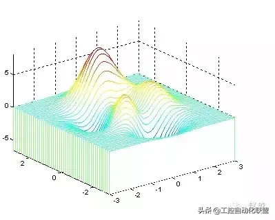
下列命令产生在y方向的水流效果:
[x,y,z]=peaks;
waterfall(x',y',z');
axis([-inf inf -inf inf -inf inf]);
meshc同时画出网状图与等高线:
[x,y,z]=peaks;
meshc(x,y,z);
axis([-inf inf -inf inf -inf inf]);
surfc同时画出曲面图与等高线:
[x,y,z]=peaks;
surfc(x,y,z);
axis([-inf inf -inf inf -inf inf]);
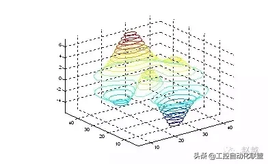
contour3画出曲面在三度空间中的等高线:
contour3(peaks, 20);
axis([-inf inf -inf inf -inf inf]);
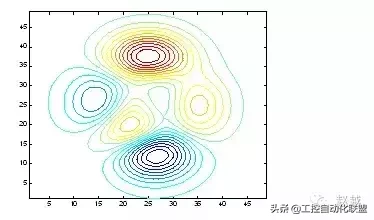
contour画出曲面等高线在XY平面的投影:
contour(peaks, 20);
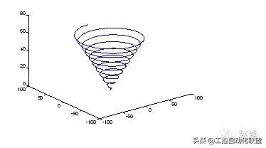
plot3可画出三度空间中的曲线:
t=linspace(0,20*pi, 501);
plot3(t.*sin(t), t.*cos(t), t);
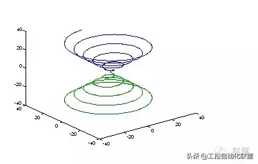
亦可同时画出两条三度空间中的曲线:
t=linspace(0, 10*pi, 501);
plot3(t.*sin(t), t.*cos(t), t, t.*sin(t), t.*cos(t), -t);
3. 三维网图的高级处理
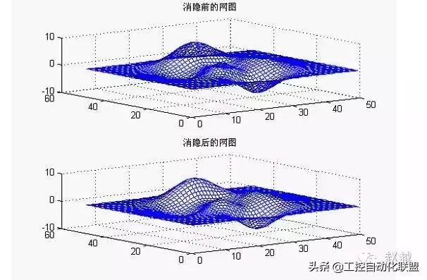
3a. 消隐处理
例.比较网图消隐前后的图形
z=peaks(50);
subplot(2,1,1);
mesh(z);
title('消隐前的网图')
hidden off
subplot(2,1,2)
mesh(z);
title('消隐后的网图')
hidden on
colormap([0 0 1])
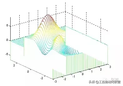
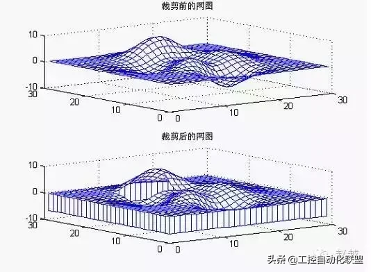
3b. 裁剪处理
利用不定数NaN的特点,可以对网图进行裁剪处理
例.图形裁剪处理
P=peaks(30);
subplot(2,1,1);
mesh(P);
title('裁剪前的网图')
subplot(2,1,2);
P(20:23,9:15)=NaN*ones(4,7); %剪孔
meshz(P) %垂帘网线图
title('裁剪后的网图')
colormap([0 0 1]) %蓝色网线
4. 三维旋转体的绘制
为了一些专业用户可以更方便地绘制出三维旋转体,MATLAB专门提供了2个函数:柱面函数cylinder和球面函数sphere
(1) 柱面图
柱面图绘制由函数cylinder实现.
[X,Y,Z]=cylinder(R,N) 此函数以母线向量R生成单位柱面.母线向量R是在单位高度里等分刻度上定义的半径向量.N为旋转圆周上的分格线的条数.可以用surf(X,Y,Z)来表示此柱面.
[X,Y,Z]=cylinder(R)或[X,Y,Z]=cylinder此形式为默认N=20且R=[1 1]
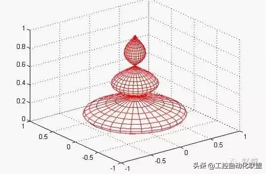
例.柱面函数演示举例
x=0:pi/20:pi*3;
r=5+cos(x);
[a,b,c]=cylinder(r,30);
mesh(a,b,c)
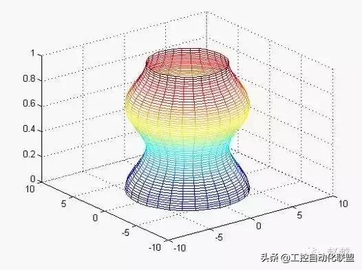
例.旋转柱面图.
r=abs(exp(-0.25*t).*sin(t));
t=0:pi/12:3*pi;
r=abs(exp(-0.25*t).*sin(t));
[X,Y,Z]=cylinder(r,30);
mesh(X,Y,Z)
colormap([1 0 0])
(2) 球面图
球面图绘制由函数sphere来实现
[X,Y,Z]=sphere(N) 此函数生成3个(N+1)*(N+1)的矩阵,利用函数 surf(X,Y,Z) 可产生单位球面.
[X,Y,Z]=sphere 此形式使用了默认值N=20.
Sphere(N) 只是绘制了球面图而不返回任何值.
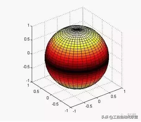
例.绘制地球表面的气温分布示意图.
[a,b,c]=sphere(40);
t=abs(c);
surf(a,b,c,t);
axis('equal') %此两句控制坐标轴的大小相同.
axis('square')
colormap('hot')
来源:工控自动化专家


 /5
/5